
728x90
SMALL
pytorch는 딥러닝/머신러닝용 라이브러리=python으로 사용할 수 있도록 warpping한 언어에 해당
torch를 이용해서 프로그래밍 해야하는데 지금은 python이라는 언어를 이용해서 해결
1. 선형회귀(Linear Regression)
import torch
import torch.optim as optim #최적화 알고리즘# (x1,y1)=(1,1), (x2,y2)=(2,2), (x3,y3)=(3,3)
x_train = torch.FloatTensor([[1], [2], [3]]) #FloatTensor를 이용하여 값 할당
y_train = torch.FloatTensor([[1], [2], [3]])# requires_grad=True 학습에 사용하겠다는 의미
W = torch.zeros(1, requires_grad=True) #사이즈가 1인 0으로 채운 변수를 할당함
print(W)# requires_grad 학습에 사용하겠다는 의미
b = torch.zeros(1, requires_grad=True)
print(b)# 학습 모델에 해당됨
hypothesis = x_train * W + b
print(hypothesis)tensor([0.],
[0.],
[0.]], grad_fn=<AddBackward0>)
# cost 값이 0에 가까워져야 가설함수가 제대로 학습된 것임
cost = torch.mean((hypothesis - y_train) ** 2)
print(cost)//GD-> 자동으로 W,b구하기--> Optimizer사용
# 최적화 방법론으로 SGD (Stochastic Gradient Descent) 를 사용하겠다고 설정
# learning rate => lr = 0.01
# W_t+1 := W_t - alpha*d/dw*cost(w)
optimizer = optim.SGD([W, b], lr=0.01)# 옵티마이저 초기화
optimizer.zero_grad()
# cost계산 !!! -> 미분값계산해서 W갱신
cost.backward()
# 옵티마이저 갱신
optimizer.step()
전체
# 데이터
x_train = torch.FloatTensor([[1], [2], [3]])
y_train = torch.FloatTensor([[1], [2], [3]])
# 모델 초기화
W = torch.zeros(1, requires_grad=True)
b = torch.zeros(1, requires_grad=True)
# optimizer 설정
optimizer = optim.SGD([W, b], lr=0.01)

nb_epochs = 1000
for epoch in range(nb_epochs + 1):

    # H(x) 계산
    hypothesis = x_train * W + b

    # cost 계산
    cost = torch.mean((hypothesis - y_train) ** 2)

    # cost로 H(x) 개선
    optimizer.zero_grad()
    cost.backward()
    optimizer.step()

    # 100번마다 로그 출력
    if epoch % 100 == 0:
        print('Epoch {:4d}/{} W: {:.3f}, b: {:.3f} Cost: {:.6f}'.format(
            epoch, nb_epochs, W.item(), b.item(), cost.item()
        ))
2. 비용 최소화하기 (Minimizing Cost)
# 시각화용 라이브러리
import matplotlib.pyplot as plt

import numpy as np
import torch
import torch.optim as optimx_train = torch.FloatTensor([[1], [2], [3]])
y_train = torch.FloatTensor([[1], [2], [3]]# Data
plt.scatter(x_train, y_train)
# Best-fit line
xs = np.linspace(1, 3, 1000) #1에서부터 3까지를 1000등분
plt.plot(xs, xs)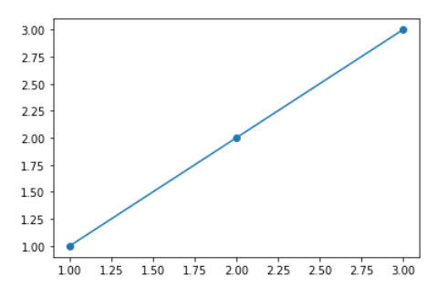
# -5 ~ 7 사이를 1000등분해서 w_l
# list <= 순차적으로 데이터를 담는 추상자료형
# w_list
W_l = np.linspace(-5, 7, 1000)
# cost list
cost_l = []
for W in W_l:
hypothesis = W * x_train
cost = torch.mean((hypothesis - y_train) ** 2)
cost_l.append(cost.item())plt.plot(W_l, cost_l) #2d그림을 그리겠다
plt.xlabel('$W$') #x축 라벨
plt.ylabel('Cost') #y축 라벨
plt.show()#그림 그리기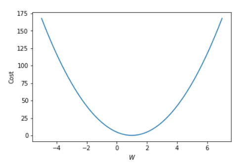
GD손으로..
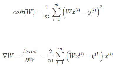
gradient = torch.sum((W * x_train - y_train) * x_train) #2/m은 생략가능
print(gradient)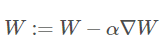
lr = 0.1 # lr = learning rate = 알파 (alpha)
W -= lr * gradient # w = w - lr * gradient
print(W)모델 학습(직접 유도한 수식에 의한, 수동미분)
# 데이터
x_train = torch.FloatTensor([[1], [2], [3]])
y_train = torch.FloatTensor([[1], [2], [3]])
# 모델 초기화
W = torch.zeros(1)
# learning rate 설정
lr = 0.1
nb_epochs = 10
for epoch in range(nb_epochs + 1):
# H(x) 계산
hypothesis = x_train * W
# cost gradient 계산
cost = torch.mean((hypothesis - y_train) ** 2)
gradient = torch.sum((W * x_train - y_train) * x_train)
print('Epoch {:4d}/{} W: {:.3f}, Cost: {:.6f}'.format(
epoch, nb_epochs, W.item(), cost.item()
))
# cost gradient로 H(x) 개선
W -= lr * gradient
3. 다중 선형 회귀(Multivariate Linear Regression)
import torch
import torch.optim as optim


# 데이터
x1_train = torch.FloatTensor([[73], [93], [89], [96], [73]])
x2_train = torch.FloatTensor([[80], [88], [91], [98], [66]])
x3_train = torch.FloatTensor([[75], [93], [90], [100], [70]])
y_train = torch.FloatTensor([[152], [185], [180], [196], [142]])

# 모델 초기화- 단순데이터를 이용한 모델학습
w1 = torch.zeros(1, requires_grad=True)
w2 = torch.zeros(1, requires_grad=True)
w3 = torch.zeros(1, requires_grad=True)
b = torch.zeros(1, requires_grad=True)
# optimizer 설정
optimizer = optim.SGD([w1, w2, w3, b], lr=1e-5)

nb_epochs = 1000
for epoch in range(nb_epochs + 1):

    # H(x) 계산
    hypothesis = x1_train * w1 + x2_train * w2 + x3_train * w3 + b

    # cost 계산
    cost = torch.mean((hypothesis - y_train) ** 2)

    # cost로 H(x) 개선
    optimizer.zero_grad()
    cost.backward()
    optimizer.step()

    # 100번마다 로그 출력
    if epoch % 100 == 0:
        print('Epoch {:4d}/{} w1: {:.3f} w2: {:.3f} w3: {:.3f} b: {:.3f} Cost: {:.6f}'.format(
            epoch, nb_epochs, w1.item(), w3.item(), w3.item(), b.item(), cost.item()
))x_train = torch.FloatTensor([[73, 80, 75],
[93, 88, 93],
[89, 91, 90],
[96, 98, 100],
[73, 66, 70]])
y_train = torch.FloatTensor([[152], [185], [180], [196], [142]])
# 모델 초기화 -행렬 데이터를 이용한 모델학습
W = torch.zeros((3, 1), requires_grad=True) #3X1짜리 W
b = torch.zeros(1, requires_grad=True)
# optimizer 설정
optimizer = optim.SGD([W, b], lr=1e-5)
nb_epochs = 20
for epoch in range(nb_epochs + 1):
# H(x) 계산
# Matrix 연산!!
hypothesis = x_train.matmul(W) + b # or .mm or @
# cost 계산
cost = torch.mean((hypothesis - y_train) ** 2)
# cost로 H(x) 개선
optimizer.zero_grad()
cost.backward()
optimizer.step()
# 100번마다 로그 출력
print('Epoch {:4d}/{} hypothesis: {} Cost: {:.6f}'.format(
epoch, nb_epochs, hypothesis.squeeze().detach(), cost.item()
))728x90
LIST
'AI' 카테고리의 다른 글
| 실습- MINST (0) | 2022.10.03 |
|---|---|
| 다중 퍼셉트론(이론) (0) | 2022.10.03 |
| 선형분류 실습 (0) | 2022.10.02 |
| 선형분류(Linear Classification) 이론 (0) | 2022.10.02 |
| 선형 회귀(Linear Regression) (0) | 2022.09.30 |